Getting Started — Your First Weathermap
This guide walks you from an empty dashboard to a live weathermap showing traffic between two devices. It should take about 10 minutes. The screenshots below were taken on Grafana 12.4 with a Prometheus data source — other supported versions look nearly identical.
Prerequisites
- Grafana 11.0.0 or later with the Network Weathermap NG panel installed (see Installation).
- At least one data source (Prometheus, InfluxDB, Zabbix, or any Grafana-compatible source) returning time-series interface counters (e.g. bits/sec in and out of an interface).
1. Create the panel
- Open or create a dashboard and click Add → Visualization.
- In the visualization picker, search for Network Weathermap and select it.
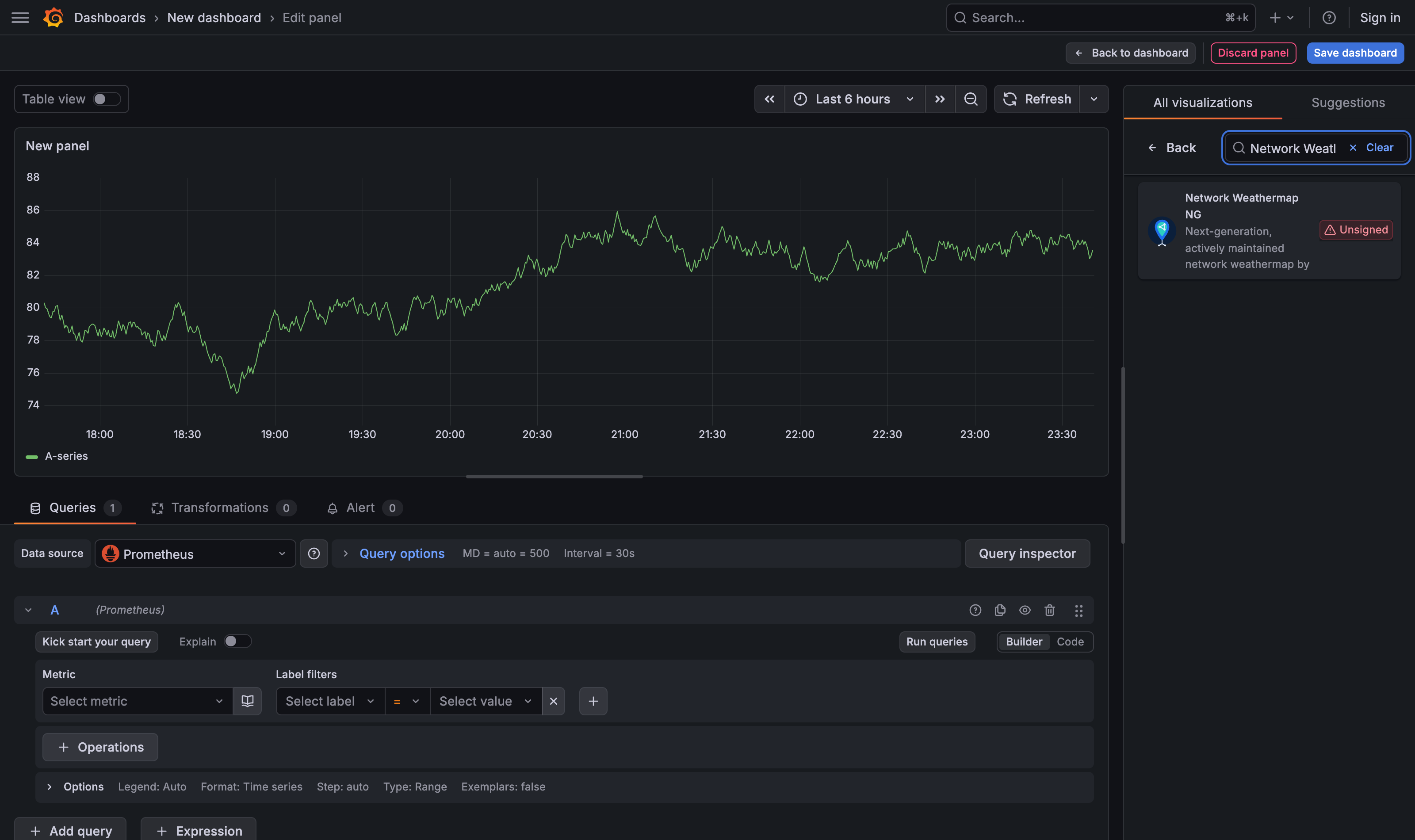
An Unsigned badge only appears on local development builds — the plugin installed from the Grafana catalog is signed.
You now have a weathermap canvas with a small starter map (two example nodes, Node A and Node B, already connected by a link) and, on the right, the panel options under Network Weathermap NG.
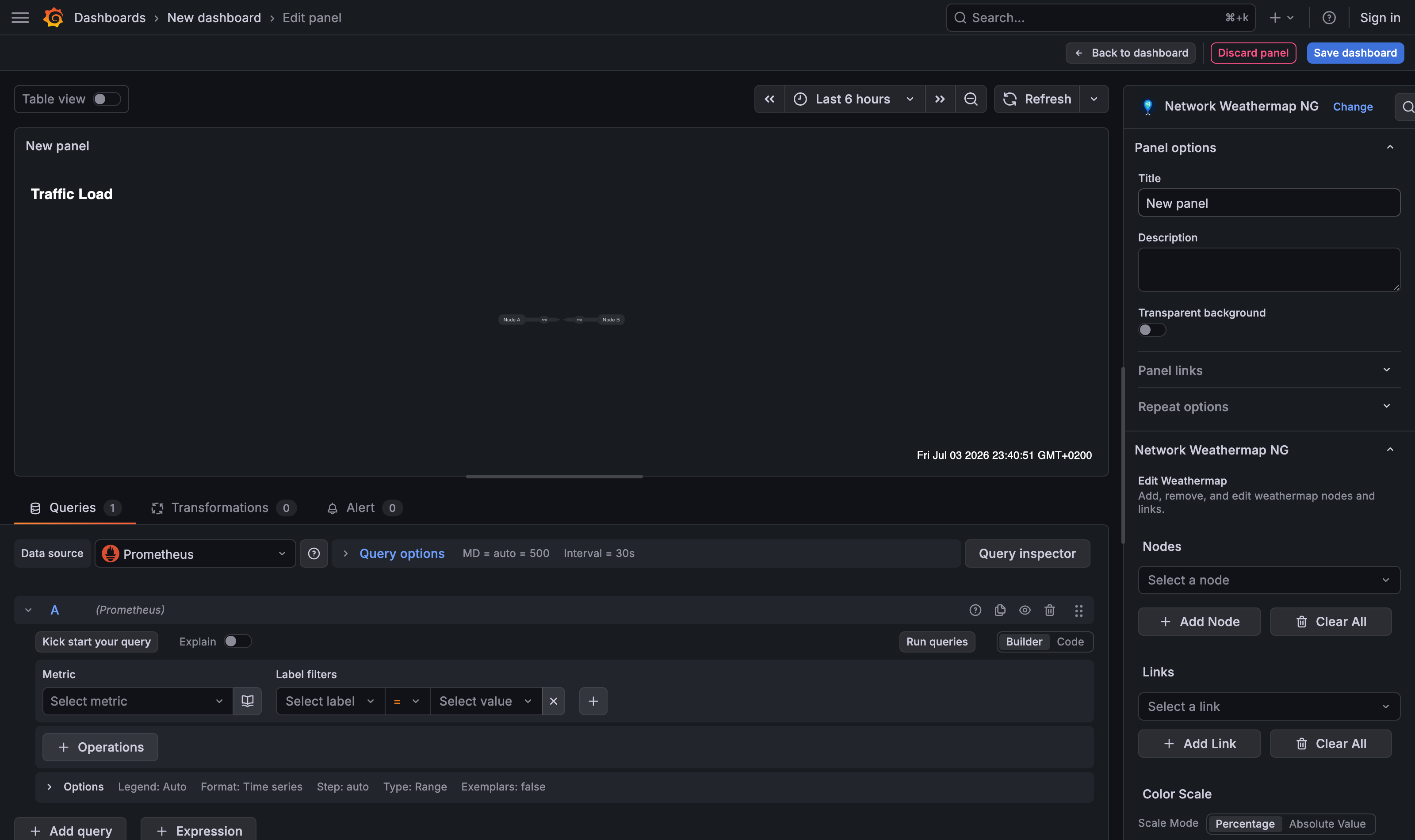
The map has two states:
| State | How you get there | What you can do |
|---|---|---|
| Edit mode | The panel edit screen (where you are now) | Add/move/delete nodes and links, drag VIAs, zoom |
| View mode | A saved dashboard | Hover for tooltips, click nodes/links that have dashboard links |
2. Add your data queries
Weathermap doesn't query data itself — it reuses the panel's queries. In the Queries tab (below the panel), add the metrics you want to visualize. A typical link needs two series:
- Outbound (A → Z) — e.g. interface bits sent
- Inbound (Z → A) — e.g. interface bits received
Give queries readable names
Weathermap identifies a series by its display name. Use a query refId or a transform/legend so each series has a clear, unique name — you'll pick it from a dropdown later. In Prometheus, set Options → Legend → Custom on each query, as below.
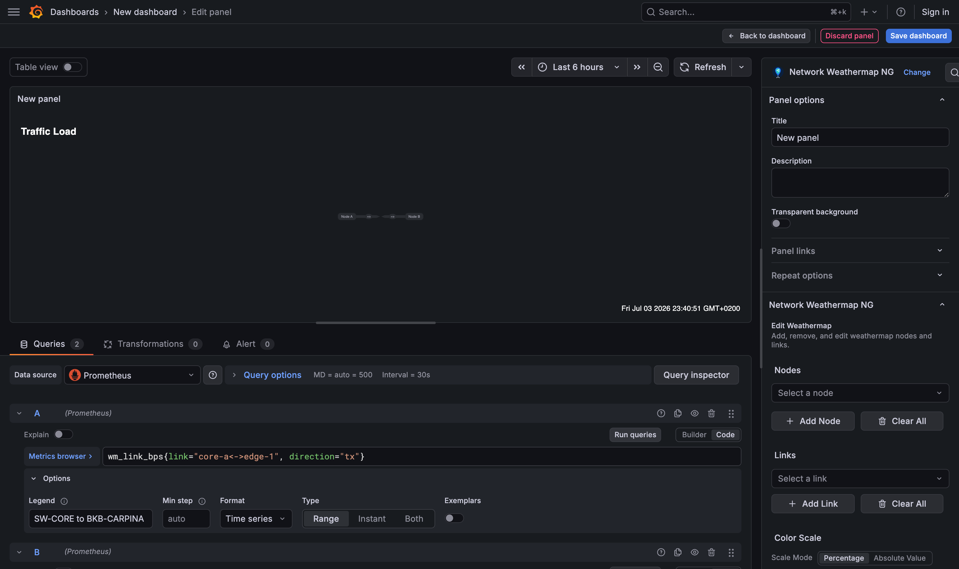
Here query A is the outbound series with legend SW-CORE to BKB-CARPINA, and query B is the inbound series with legend BKB-CARPINA to SW-CORE. Click Run queries so the panel sees the data.
3. Add your devices (nodes)
- In the panel options, open the Nodes section.
- Click Add Node (or pick one of the starter nodes from the dropdown). The node's form opens.
- Set its Label (e.g.
SW-CORE) and, if you like, exact X/Y coordinates. - Or simply drag the node on the canvas to position it. (Hold nothing — just click-drag in edit mode.)
- Repeat for a second device (e.g.
BKB-CARPINA).
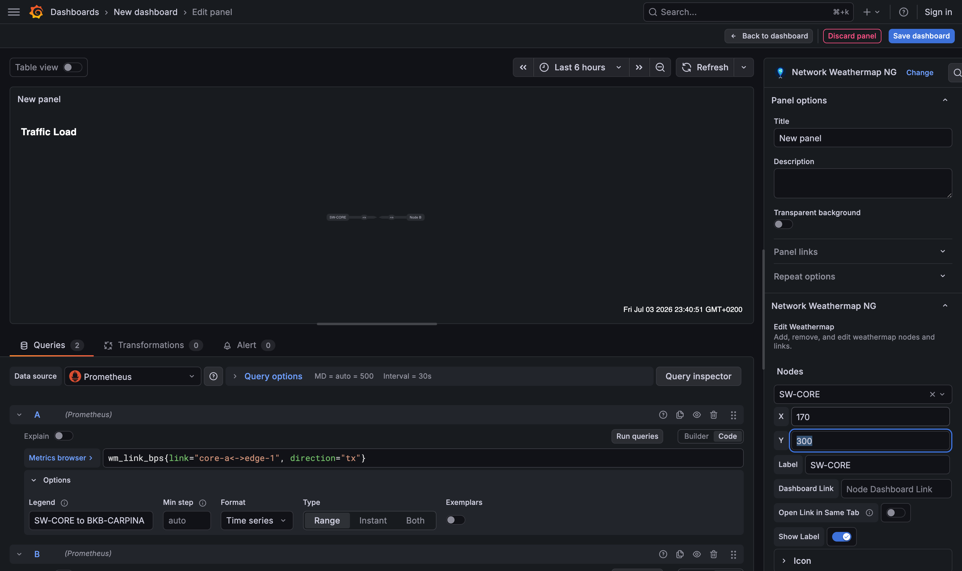
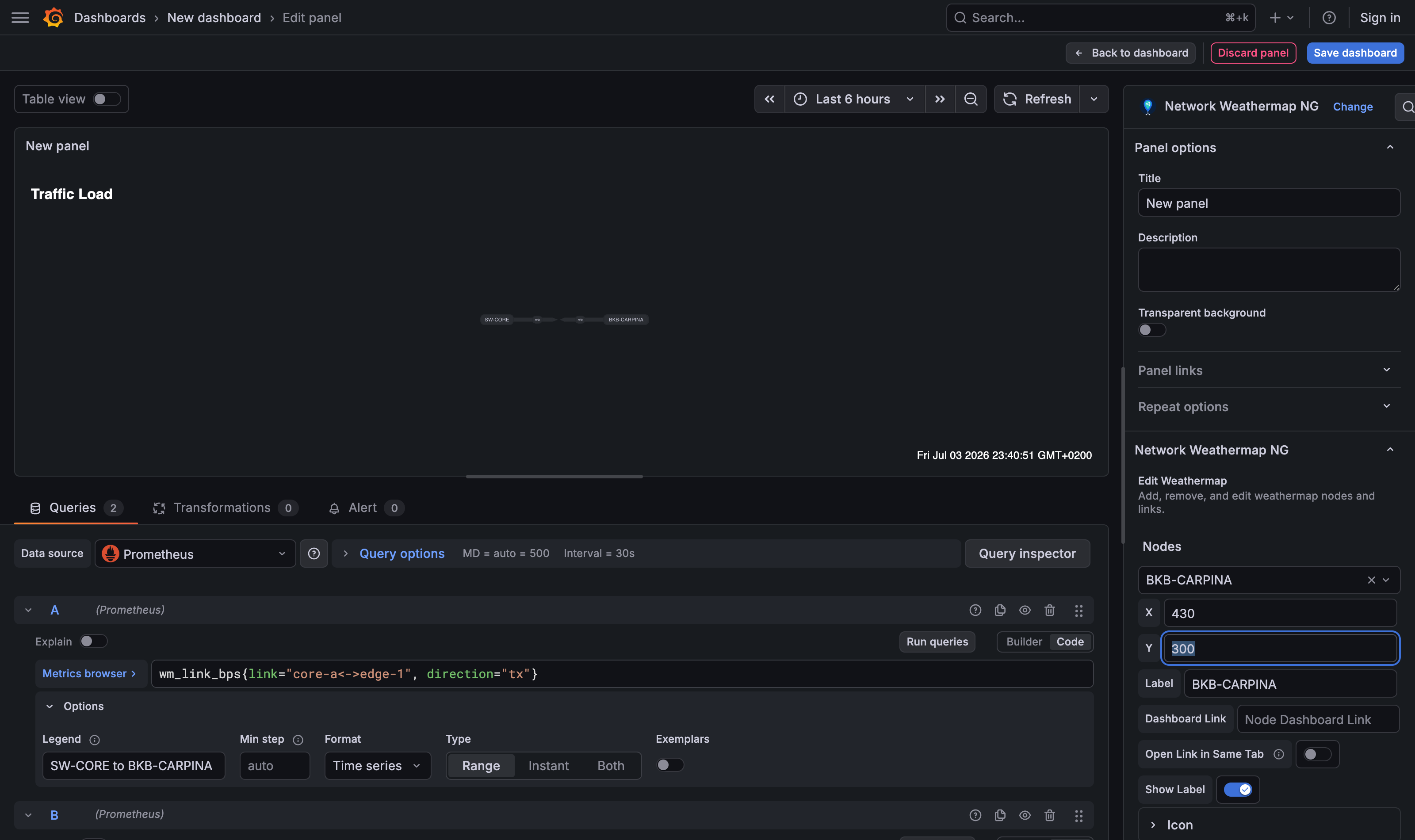
See Nodes (Devices) for icons, status coloring, and per-node tooltips.
4. Connect them with a link
- Open the Links section and click Add Link (or select the starter link from the dropdown).
- Set A Side to your first node and Z Side to the second.
- Under A Side Options, set A Side Query to your outbound series and, optionally, A Bandwidth # (or A Bandwidth Query) to the link capacity so utilization can be shown as a percentage.
- Under Z Side Options, set Z Side Query to your inbound series and its bandwidth.
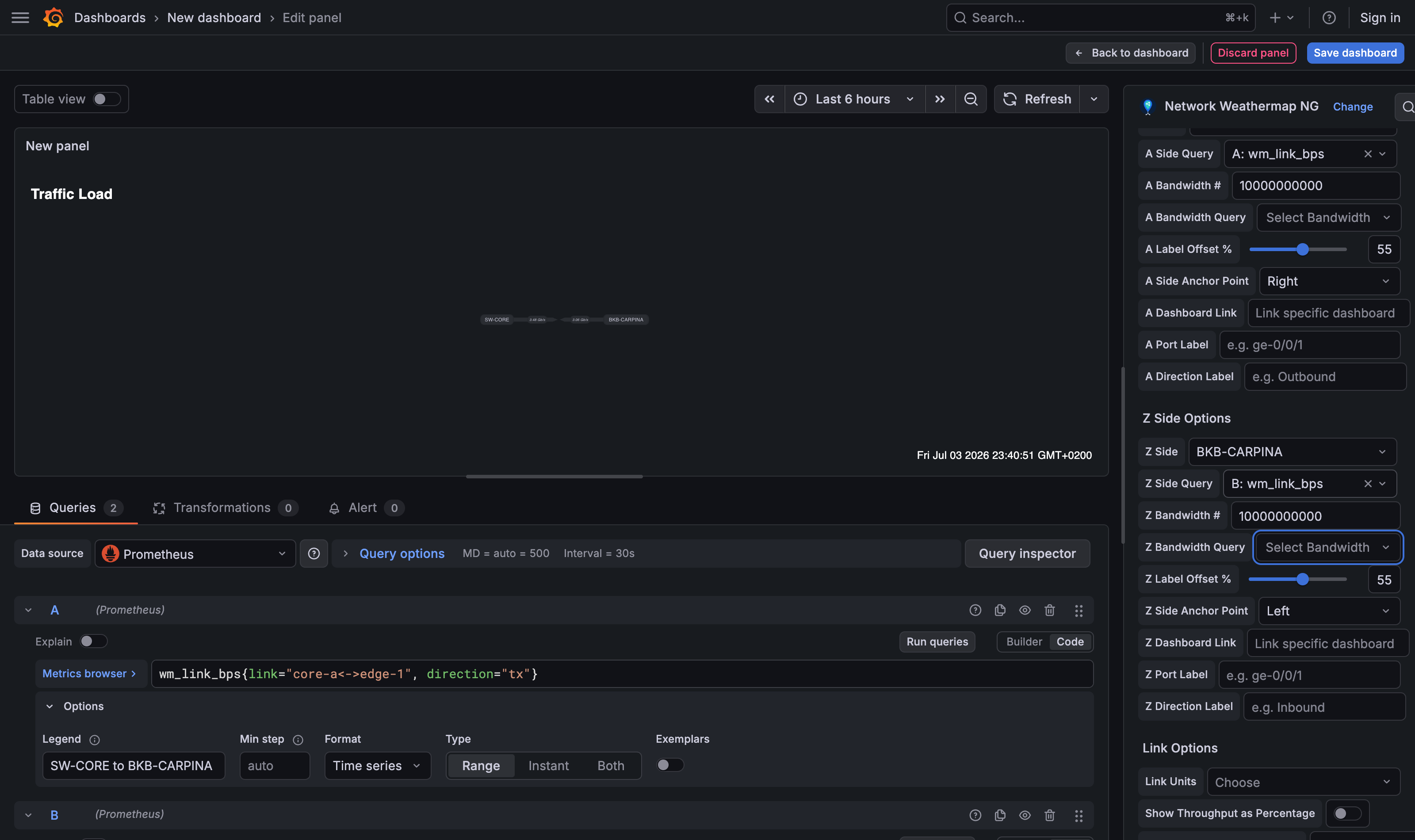
The link now colors itself according to utilization, arrows show direction, and the live values render on the map (10000000000 = 10 Gbps capacity per side in this example). See Links for units, direction labels, and more.
5. Set the color scale
- Open the Color Scale section (panel options).
- Add thresholds mapping a percentage (or absolute value) to a color — for example
0% → green,50% → yellow,80% → orange,95% → red.
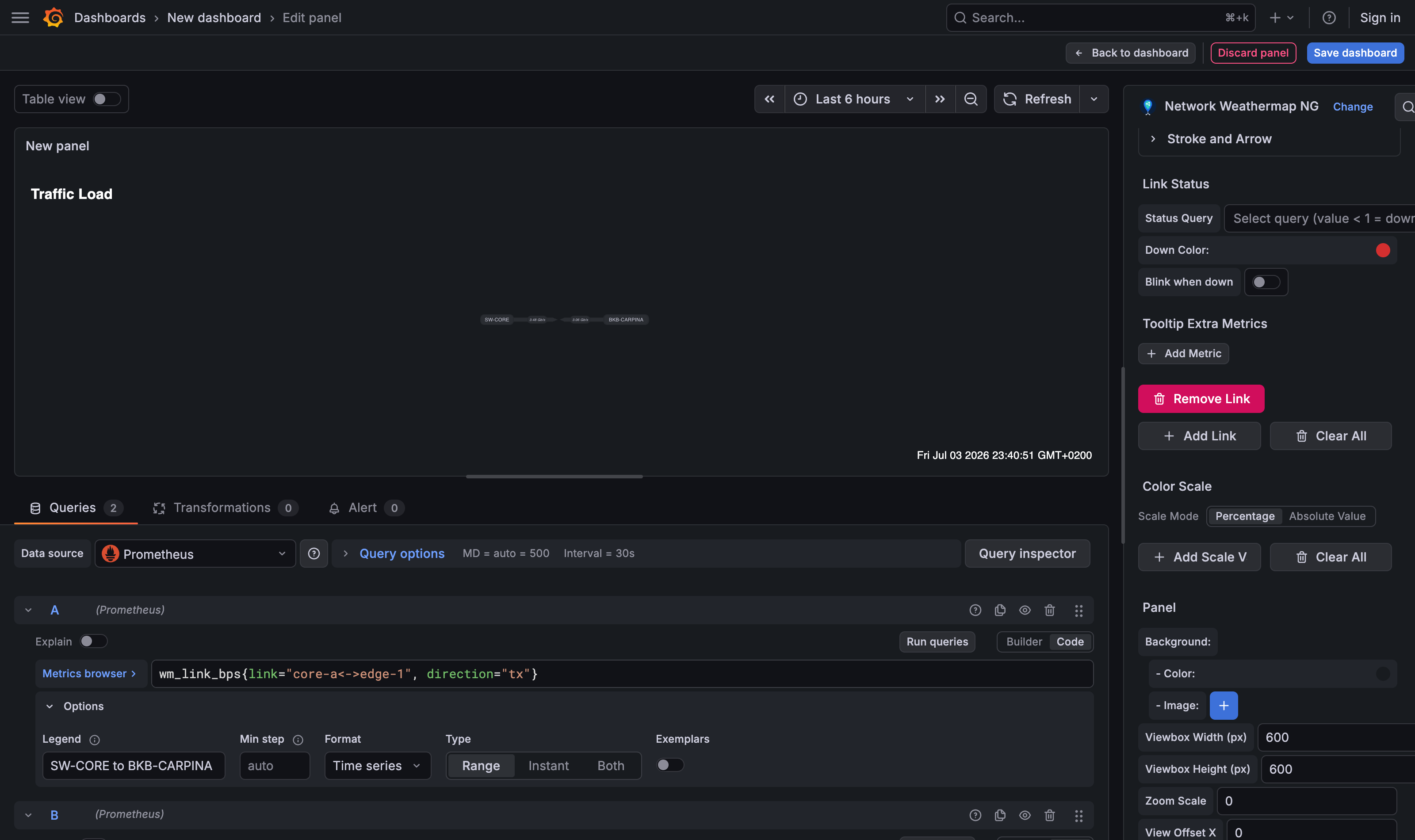
Links and the legend now reflect these bands.
6. Save and use it
- Click Save dashboard, give it a name, and exit the panel editor.
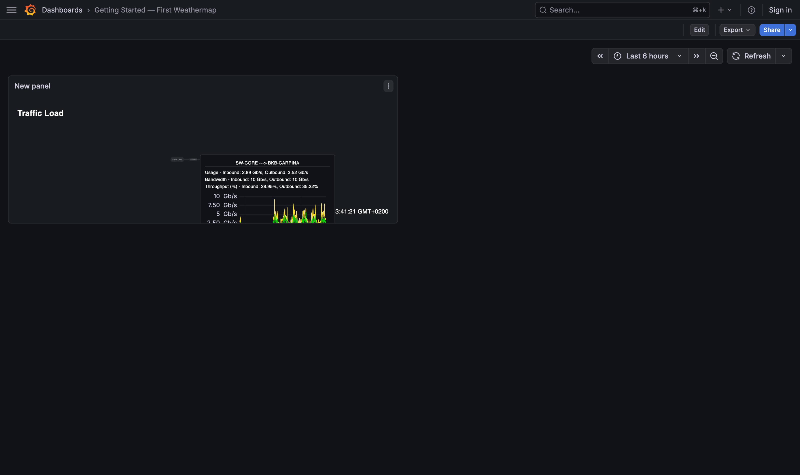
- In view mode, hover a link to see a tooltip with usage, bandwidth, throughput %, and a mini time-series graph.
- Hover a node to see any extra metrics you configured.
Where to go next
- Nodes (Devices) — icons, status colors, node tooltips, dashboard links
- Links — queries, units, direction labels, port labels, parallel links, VIAs
- Panel Options — background image, value display modes, timeline slider, tooltips
- Interactions & Editing — pan/zoom/select on every OS, VIA editing, export
- Use Cases — end-to-end scenarios (capacity planning, incident retros, floor plans)