Data Sources

The weathermap is datasource-agnostic: it reads whatever time series Grafana hands it. Any datasource that returns a time field and a numeric value field works — Prometheus, InfluxDB, Elasticsearch, Zabbix, PostgreSQL, MySQL, and most others.

The one rule that matters everywhere

The panel binds link sides to series by display name — the name you see in the link editor's A/B Side Query dropdown. Keep your legends/aliases stable: renaming a series later breaks the binding, and duplicate display names resolve to the first matching series. Always pick series from the dropdown rather than typing names by hand.

The universal process

Whatever the datasource, building a weathermap dashboard is the same five steps:

1. Provision the datasource in Grafana (Connections → Data sources).
2. Add the panel queries — typically one series per link side (A = transmit, Z = receive), one per link.
3. Name each series stably with the datasource's legend/alias feature (examples per source below).
4. Bind the series: in the panel editor open Links, select a link, and pick the series in the A Side Query and Z Side Query dropdowns.
5. Set bandwidth and thresholds so the color scale means something.

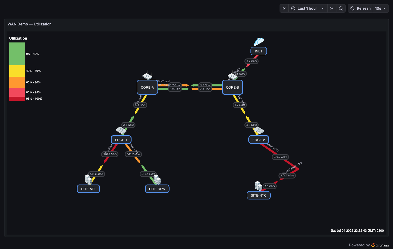
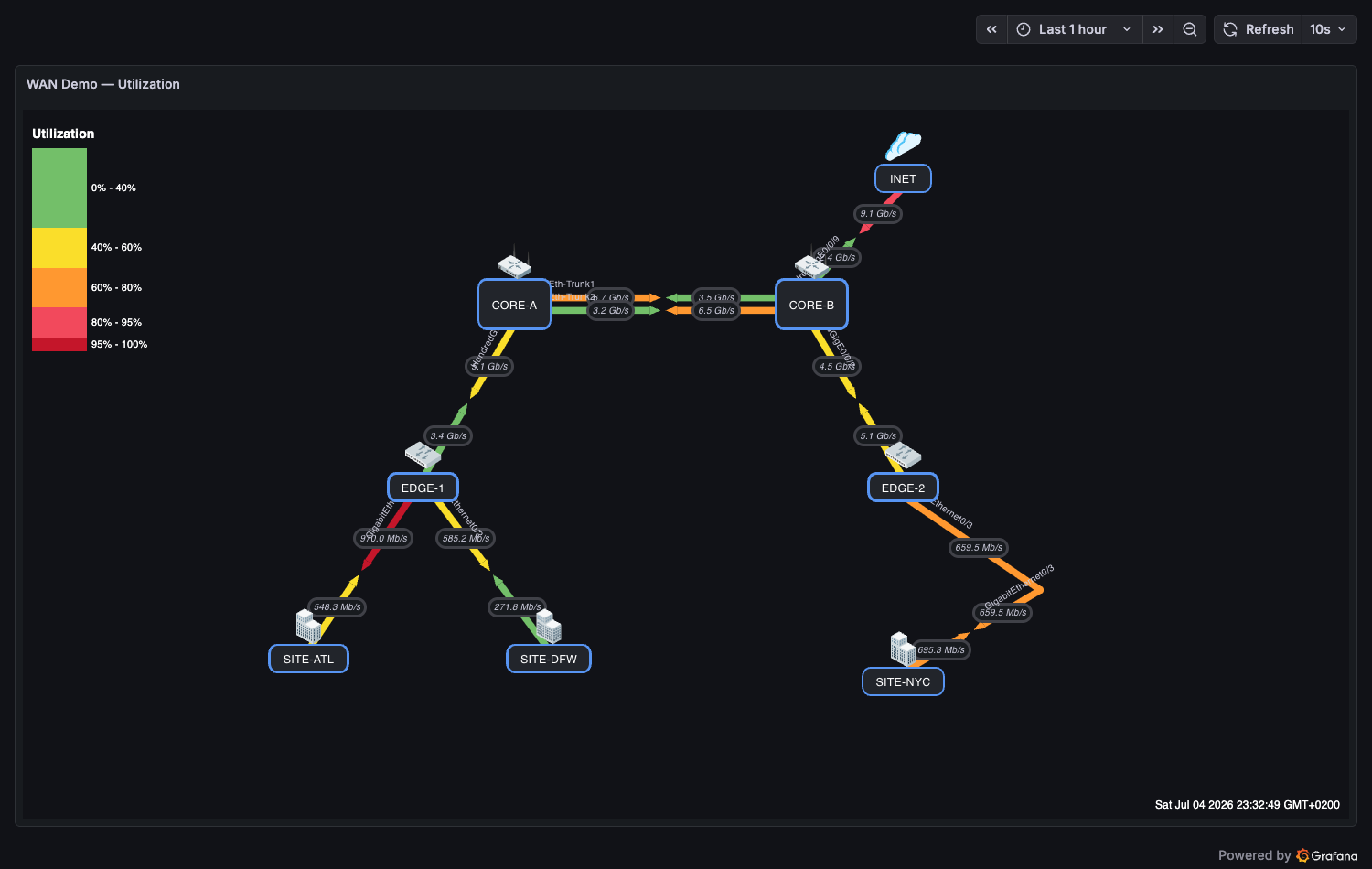
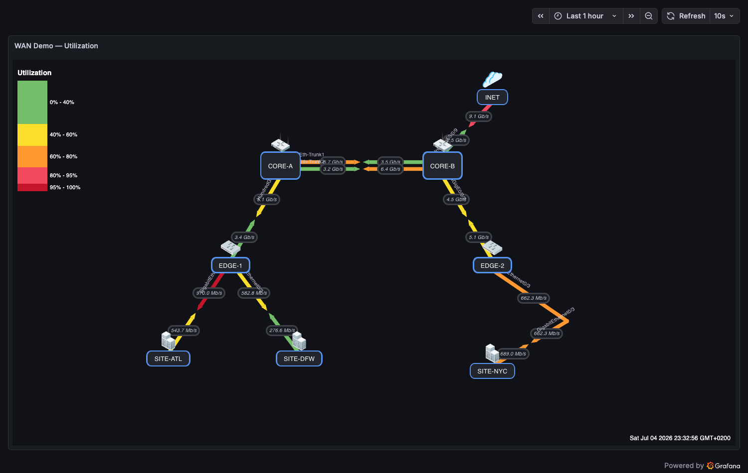
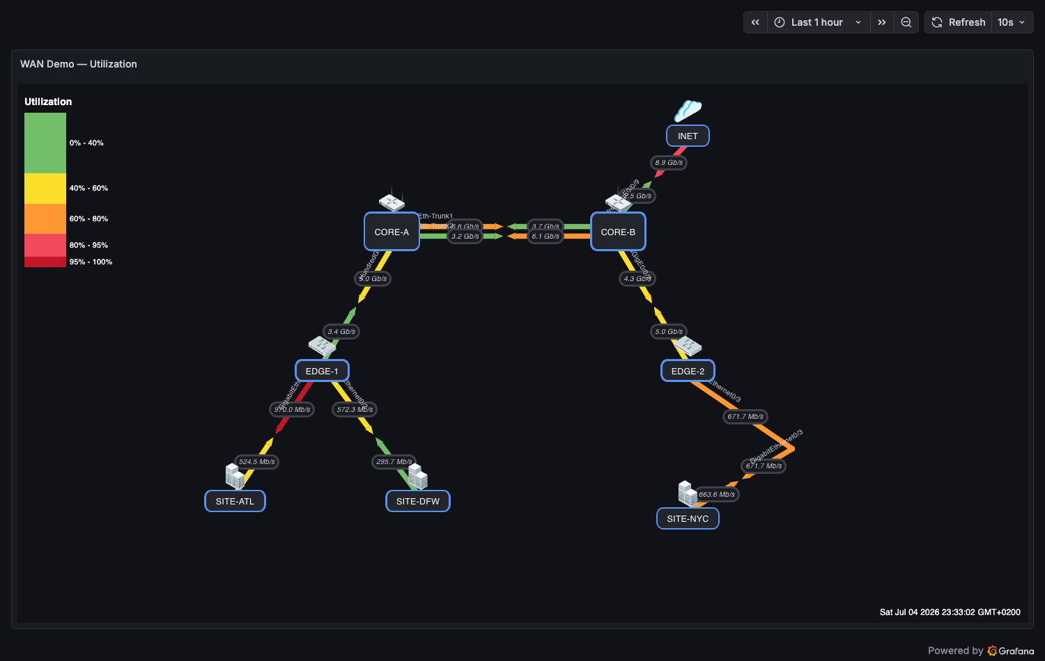
The demo stack (cd testing && docker compose up --build) runs the same simulated WAN metrics through Prometheus, InfluxDB, Elasticsearch, Zabbix, PostgreSQL, and MySQL simultaneously — a bridge forwards the exporter's values to every backend, tagged with identical series names. Each provisioned dashboard renders the same map from the same numbers:

• WAN Demo — Utilization (Prometheus)
• WAN Demo — Utilization (InfluxDB) — one Flux query + a rename-by-regex transformation
• WAN Demo — Utilization (Elasticsearch) — one terms + date-histogram query, no transformation needed
• WAN Demo — Utilization (Zabbix) — one group/host/item wildcard query; item names are the series names, no transformation needed
• WAN Demo — Utilization (PostgreSQL) / (MySQL) — one SQL query in Time series format; the metric column names the series, no transformation needed

Open them side by side to see that the weathermap options are byte-identical — only the queries differ. testing/scripts/generate-datasource-dashboards.py regenerates the variants from the Prometheus original.

---

Prometheus

The canonical setup — all bundled demo dashboards use it.

Query (link utilization in bits/s, one direction):

wm_link_bps{device="core-a", peer="core-b", direction="tx"}

Legend: set the query's Legend field so the display name is stable and readable:

{{device}}→{{peer}} {{iface}} {{direction}}

If your source exposes counters instead of gauges, wrap with rate():

rate(ifHCOutOctets{ifName="ge-0/0/1"}[5m]) * 8

Binding: the legend text is exactly what appears in the A/B Side Query dropdowns.

Deviations: none — Prometheus is the baseline; legends map 1:1 to display names.

Link status (for the down state and traffic animation): bind a link's Status Query to an operational-status series — 0/absent renders the link down (dashed, DOWN, and, with animation on, static ✕ badges):

wm_link_status{link="core-a<->edge-1"}     # demo simulator (1 = up, 0 = down)
ifOperStatus{instance="core-switch", ifName="Gi1/0/1"}   # real SNMP equivalent

The WAN Demo — Animated Traffic Flow dashboard is driven entirely from these Prometheus series — see the animation use case for the full data path.

---

InfluxDB

Works with both query languages. The demo stack provisions InfluxDB 2.x (bucket wm, org wm) on :8086, fed by the same simulator.

Flux:

from(bucket: "wm")
  |> range(start: v.timeRangeStart, stop: v.timeRangeStop)
  |> filter(fn: (r) => r._measurement == "wm_link_bps")
  |> filter(fn: (r) => r.device == "core-a" and r.direction == "tx")
  |> aggregateWindow(every: v.windowPeriod, fn: mean, createEmpty: false)

Flux names series from the tag set (e.g. wm_link_bps {device="core-a", direction="tx", ...}). To control the display name, add:

  |> map(fn: (r) => ({ r with _field: "core-a→core-b tx" }))

InfluxQL (v1 compatibility):

SELECT mean("value") FROM "wm_link_bps"
WHERE ("device" = 'core-a' AND "direction" = 'tx') AND $timeFilter
GROUP BY time($__interval) fill(null)

Use Alias by to fix the display name: core-a→core-b tx.

Frame shape note: Influx value fields arrive named _value (Flux) or mean (InfluxQL) rather than Value — the panel resolves the value field by numeric type, not by name, so both bind cleanly. This behavior is locked by unit tests.

Deviation: single-label Flux frames display as value <series>

When a Flux query returns frames with one label, Grafana computes the display name as value <label value> — not the bare series name. Add a Rename by regex transformation (^value (.*)$ → $1) so the display names match your bindings. The demo dashboard ships exactly this transformation.

---

Elasticsearch

For metrics stored as documents (e.g. from Beats/Logstash or the demo bridge writing to the wm-metrics index on :9200).

Query setup:

• Query: Lucene filter, e.g. device:core-a AND direction:tx
• Metric: Average of your value field, e.g. bps
• Group by: Date Histogram on @timestamp (interval auto)
• Optional second group: Terms on link.keyword to fan out one query into per-link series

Alias: set the query Alias to stabilize the display name, e.g. {{term link.keyword}} tx or a literal core-a→core-b tx.

Frame shape note: ES frames often carry names like Average bps combined with the term value; whatever ends up as the display name in Grafana's legend is what the link editor's dropdown shows — pick from the dropdown and it binds.

Deviation: cap the panel's Max data points

A terms × date-histogram query multiplies buckets: many series at panel-width resolution exceeds Elasticsearch's 65,536-bucket search limit and the whole query errors. Set the panel's Max data points (Query options) so series × points stays under the limit — the demo dashboard uses 250 for its 204 series.

---

Zabbix

The Zabbix datasource plugin works with the weathermap — and the demo stack runs a full Zabbix 7.0 server (UI/API on :8081, Admin / zabbix) whose wm-sim host receives every simulated series as a trapper item, pushed by the bridge with the zabbix_sender protocol. The pattern:

1. Install and configure the Zabbix plugin datasource (the demo Grafana ships it pre-installed and provisioned).
2. Query per link side using the Group/Host/Item selectors, e.g.:
3. Group: Routers · Host: core-a · Item: Interface ge-0/0/1(): Bits sent
4. Z side: the matching Bits received item on the peer, or the same host's receive item — match your monitoring convention.
5. Zabbix's item name becomes the series display name — item names are stable by nature, which suits the binding rule well.
6. Use Functions → Alias (setAlias) in the Zabbix query editor if you want shorter dropdown names.

Deviation: disable Data alignment

The Zabbix datasource's Data alignment option (on by default) merges all returned series into a single wide frame — and the panel currently binds only a wide frame's first value field, so every other link shows n/a (tracked in #260). Set Disable data alignment in the query options; the demo dashboard ships with it disabled.

Deviation: API payload size on dense history

Pulling many items at fine granularity through the Zabbix JSON-RPC API can exhaust the web frontend's PHP memory_limit (default 128M → HTTP 500). For dense setups raise it (the demo compose sets ZBX_MEMORYLIMIT=1024M on the web container) and enable trends in the datasource (the demo uses trendsFrom: 4h) so long ranges read hourly aggregates instead of raw history.

Counters vs gauges

Zabbix network items are usually already rate-calculated (Bits sent/received deltas). If yours are raw counters, add the delta/rate processing on the Zabbix side or via the query editor functions, the same way you'd rate() in Prometheus.

---

PostgreSQL / MySQL

SQL datasources work with the weathermap like any other — the panel reads standard Grafana data frames — but SQL has two extra things to get right: the result must be time-series-shaped, and each series needs a clean display name. The demo stack provisions PostgreSQL and MySQL on :5432 / :3306, fed the same simulated series by the bridge into a wm_metrics(time, series, value) table.

Format as Time series (not Table). In the query editor set Format → Time series. Return a time column, the numeric value, and a column aliased metric — Grafana uses the metric column's value as the series name, so the weathermap binds by it verbatim (no rename transform needed, unlike InfluxDB).

PostgreSQL:

SELECT "time", value, series AS metric
FROM wm_metrics
WHERE $__timeFilter("time")
ORDER BY "time"

MySQL / MariaDB (backtick identifiers):

SELECT `time`, value, series AS metric
FROM wm_metrics
WHERE $__timeFilter(`time`)
ORDER BY `time`

If your table stores one row per interval already (like the demo), that's all you need. If you're aggregating raw samples, group by a time bucket with the datasource macro:

SELECT $__timeGroupAlias("time", '$__interval'), avg(value) AS value, series AS metric
FROM wm_metrics
WHERE $__timeFilter("time")
GROUP BY 1, series
ORDER BY 1

Frame shape note: in Time series format Grafana pivots the long result (time, metric, value) into one frame per metric value, named by it, with a single numeric value field. The panel resolves the value field by numeric type, and the frame name is the display name your links bind to — so the copied WAN map's bindings match with no transformation. Wide Table results (see below) bind each numeric column by its column name instead.

Deviation: Format as Time series, or alias every column

SQL queries default to Format as → Table, which returns one wide frame. That still works — each numeric column becomes a bindable series keyed by its column name — but you must alias every value column to the display name you want (SELECT ts, out_bps AS "core-a→core-b tx", …). The simpler path for many series is Format as → Time series with a metric column, as above. Pick from the link dropdown either way.

Deviation: value and bandwidth must share a unit

The panel computes utilization as a plain value ÷ bandwidth with no unit conversion. If your query returns a percentage, set the link's Bandwidth # to 100; if it returns bits/sec, use a bits/sec bandwidth. See Links → Queries and bandwidth.

Display names come from the metric alias

Whatever the metric column contains becomes the series display name the link editor binds to — keep it stable and unique (e.g. SITE-A→SITE-B tx). Without a metric column, Grafana names the series after the value column, and your bindings won't match.

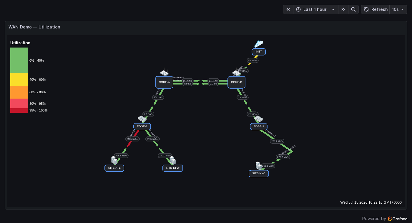
The same map, every value resolved from a PostgreSQL wm_metrics table in Time series format.

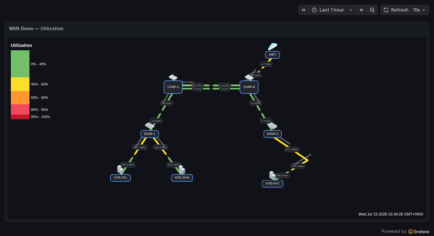
MySQL renders the identical map from the identical numbers — the bridge writes both from one source of truth.

---

Troubleshooting bindings

• Dropdown shows the series but the link stays n/a — the display name changed after binding (legend edited, label values changed). Re-pick from the dropdown.
• Two series share a name — the panel deterministically uses the first; give them distinct aliases.
• No value resolves — confirm the query returns a numeric field; string-only frames are skipped (the panel logs a console warning).