Use Cases & Scenarios
End-to-end recipes that combine the options into real dashboards. Each assumes you've completed Getting Started.
Try every scenario live
Each recipe below has a ready-made demo dashboard with simulated enterprise traffic. From a checkout of the repo:
npm install && npm run build
cd testing && docker compose up --build
then open http://localhost:3101 → Dashboards. The data generator keeps producing realistic traffic (diurnal cycles, bursts, a periodically saturating link, a flapping device) for as long as the stack runs. The screenshots on this page are captured from those dashboards.
1. WAN link utilization (two sites)
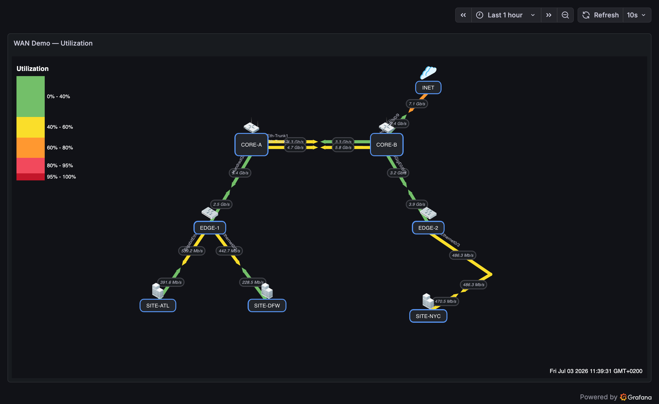
Goal: show a core uplink between two sites, colored by utilization, with clear inbound/outbound labels.
- Add nodes
SW-COREandBKB-CARPINA. - Add a link A=
SW-CORE, Z=BKB-CARPINA. - A Side Query = the outbound direction A→Z —
SW-CORE's interface bits sent; A Bandwidth # = link capacity (e.g.20000000000). - Z Side Query = the reverse direction Z→A. Use either
BKB-CARPINA's bits sent orSW-CORE's bits received (both represent Z→A) — notBKB-CARPINA's bits received, which is the same A→Z direction as the A side; Z Bandwidth # = same capacity. - Set A Direction Label =
Outbound, Z Direction Label =Inbound. - Add Port Labels (e.g.
Eth-Trunk12) so the physical interface is visible. - Give each node an Icon — the plugin bundles 680+ icons across Cisco, networking, database, computer, country flag (ISO 3166, circle style), and rack part (faceplates, PSU, fans, PDU, ports) sets, plus custom icon URLs.
- Color scale:
0→green, 50→yellow, 80→orange, 95→redwith Color Scale Mode = percent.
Hovering the link shows usage, bandwidth, throughput %, and a mini graph.
Demo: WAN Demo — Utilization — 8 devices, parallel core links, a VIA-curved long-haul, and click-through from the SITE nodes to the floor-plan dashboard.
2. Capacity planning (avg / 95th percentile)
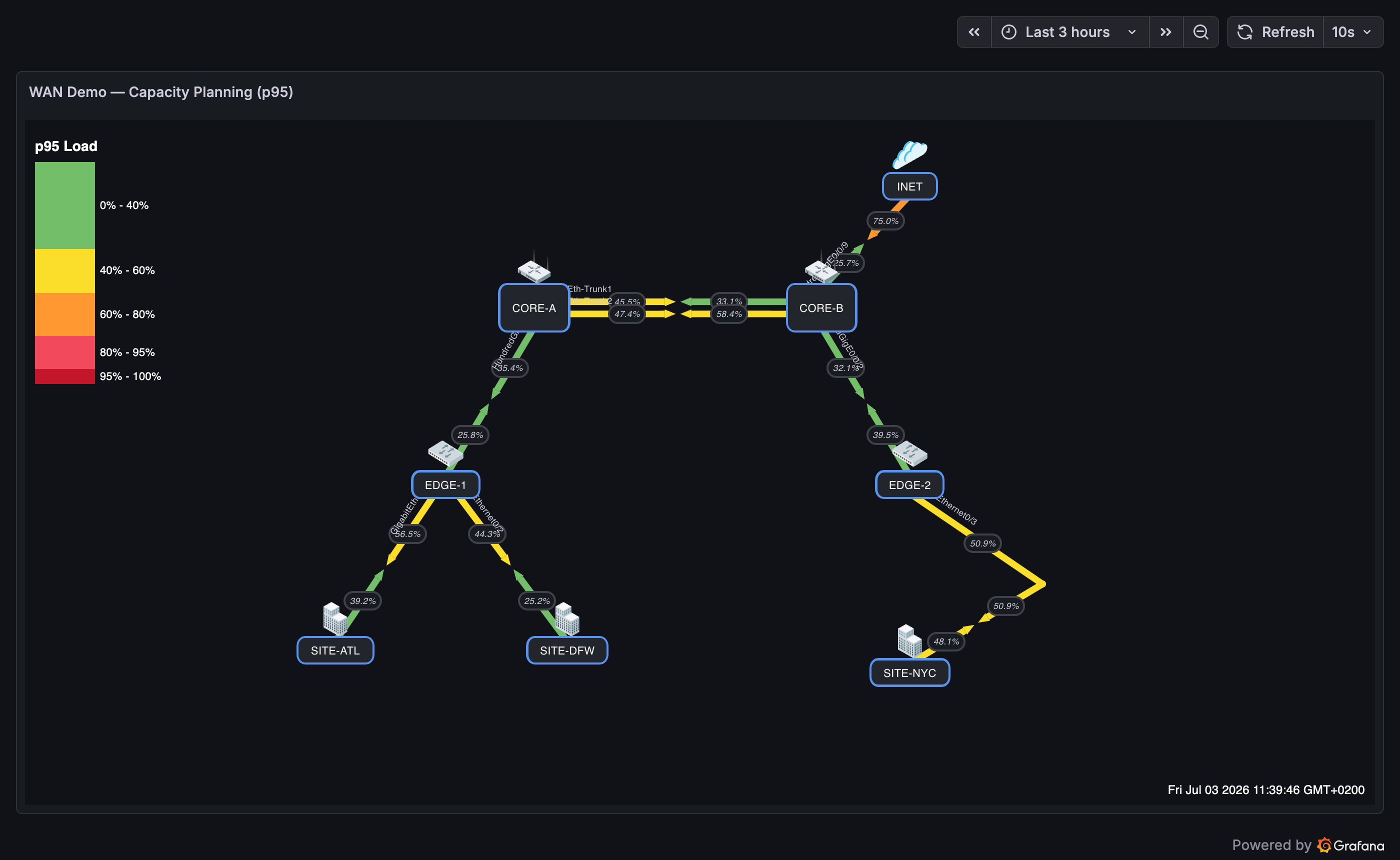
Goal: compare typical vs. peak load over a period, not just the instantaneous value.
- Build the map as in scenario 1.
- Set the dashboard time range to the period of interest (e.g. last 30 days).
- Panel Options → Value Display Mode:
- Choose 95th Percentile to size links for sustained peaks, or Average for typical load.
- Switch to Max to spot the worst-case moment.
- Compare against your color-scale bands to find links that are hot at p95.
Demo: WAN Demo — Capacity Planning (p95) — the EDGE-1 ↔ SITE-ATL link saturates for ~90 s every 7 minutes; at p95 that stays visible long after each burst passes.
3. Incident retrospective (timeline replay)
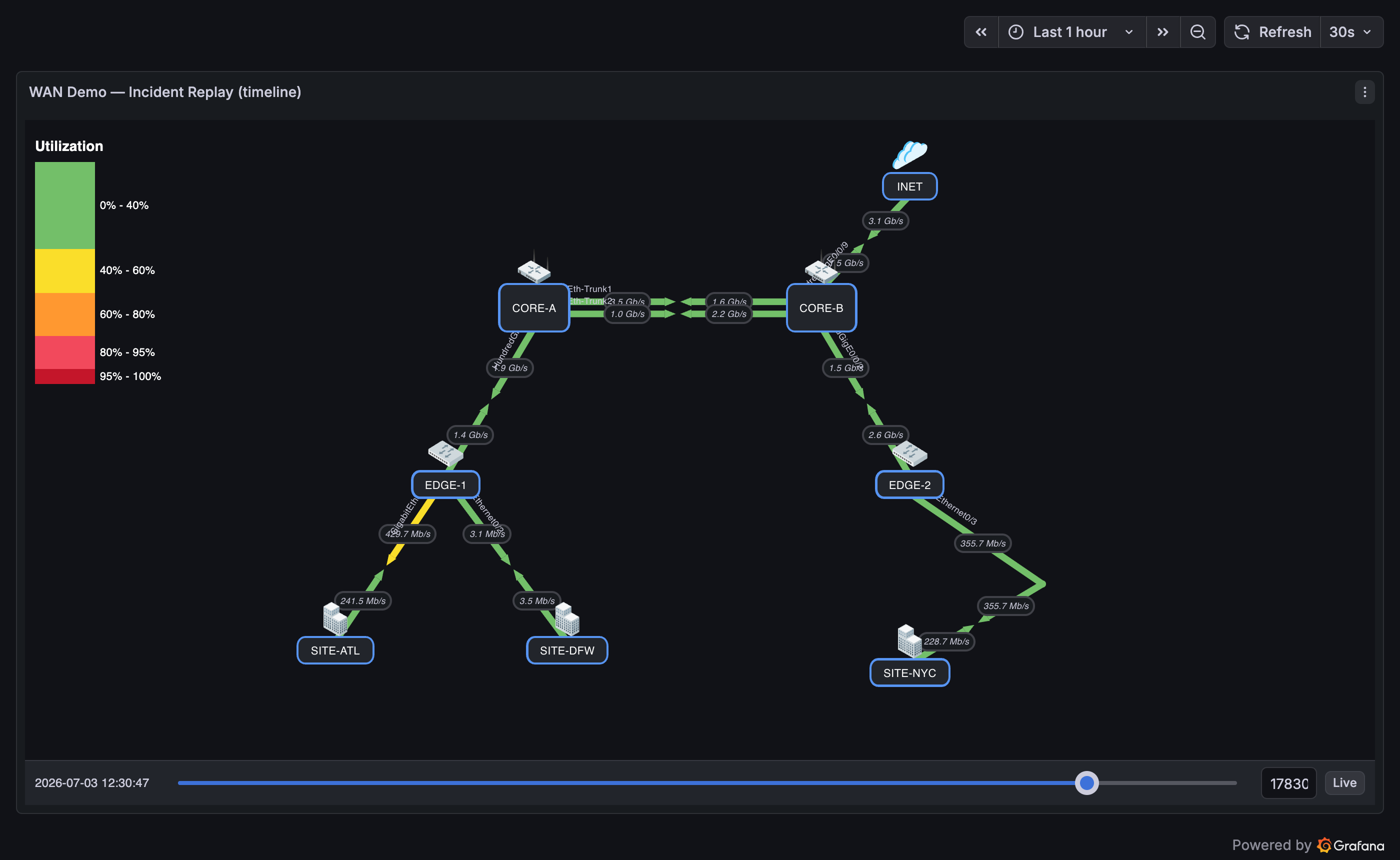
Goal: replay how the network looked during an outage window.
- Enable Panel Options → Timeline Slider.
- Set the dashboard time range to span the incident.
- In view mode, drag the slider to the moment the incident began and step forward — link colors and values update to that time.
- Use the timestamp label to correlate with alerts/logs. Press Live to return to now.
Demo: WAN Demo — Incident Replay (timeline) — SITE-DFW goes down for ~2 minutes every 10; scrub back to watch its link collapse and recover.
4. Data-center floor plan (background follows the map)
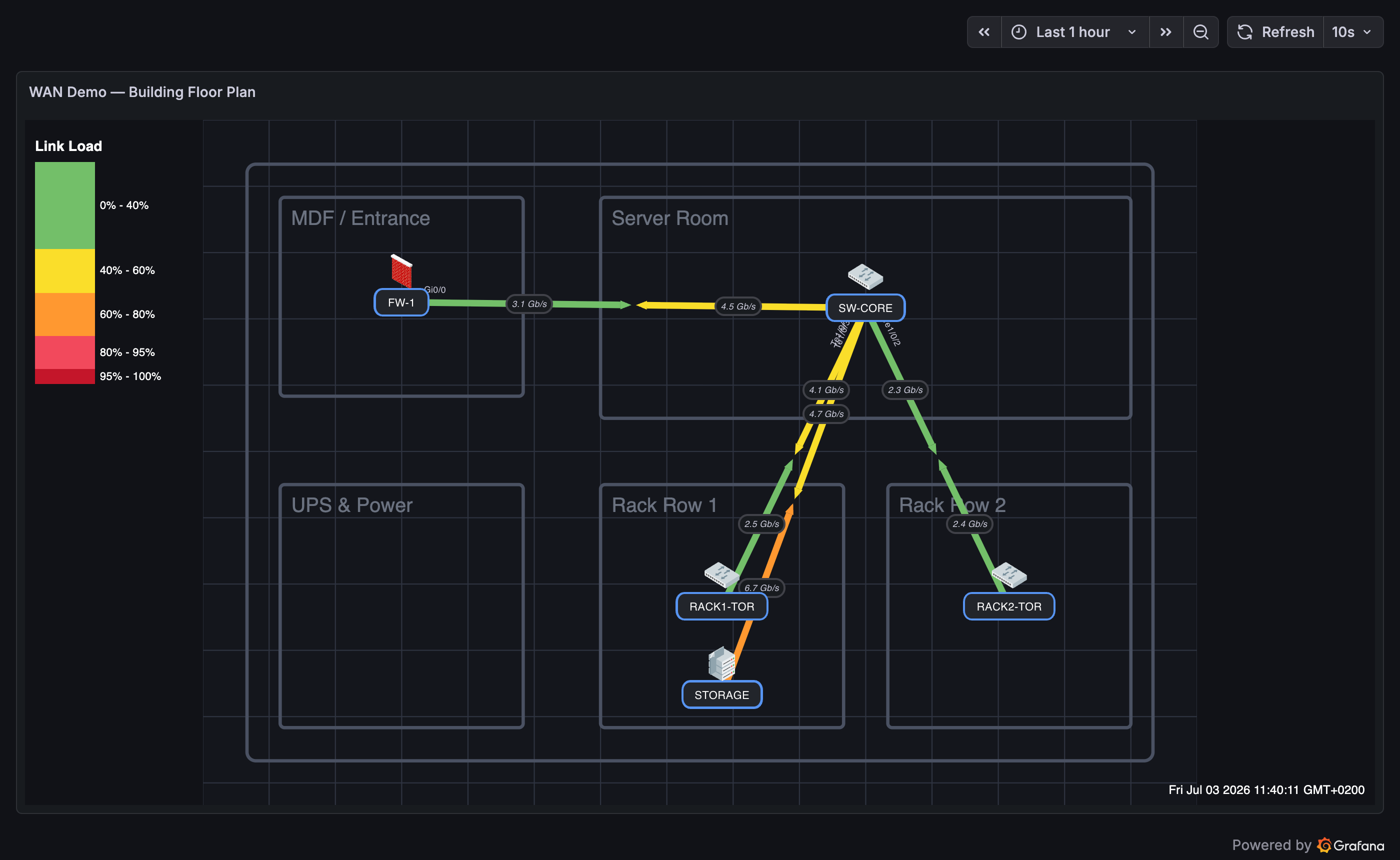
Goal: overlay devices on a floor plan or rack layout that zooms/pans with the map.
Background image hosting
The background is a URL — any http:// or https:// link works, or drop the file in Grafana's public/ folder and reference it as public/img/<name> (air-gap friendly). data: URLs are rejected. Details: Panel Options → Background.
- Panel Options → Background → Image: paste the floor-plan image URL; set Image Fit to
contain. - Enable Move With Map so the image scales and pans with the nodes.
- Place nodes on top of the plan at their physical locations; use the Grid for alignment.
- Add links to show inter-rack or inter-room traffic.
Demo: WAN Demo — Building Floor Plan — firewall, core switch, top-of-rack switches, and storage placed over a server-room plan; clicking RACK1-TOR drills into its rack port diagram (scenario 10).
5. Multi-hop path with VIAs
Goal: draw a link that routes around other elements or represents a multi-hop path.
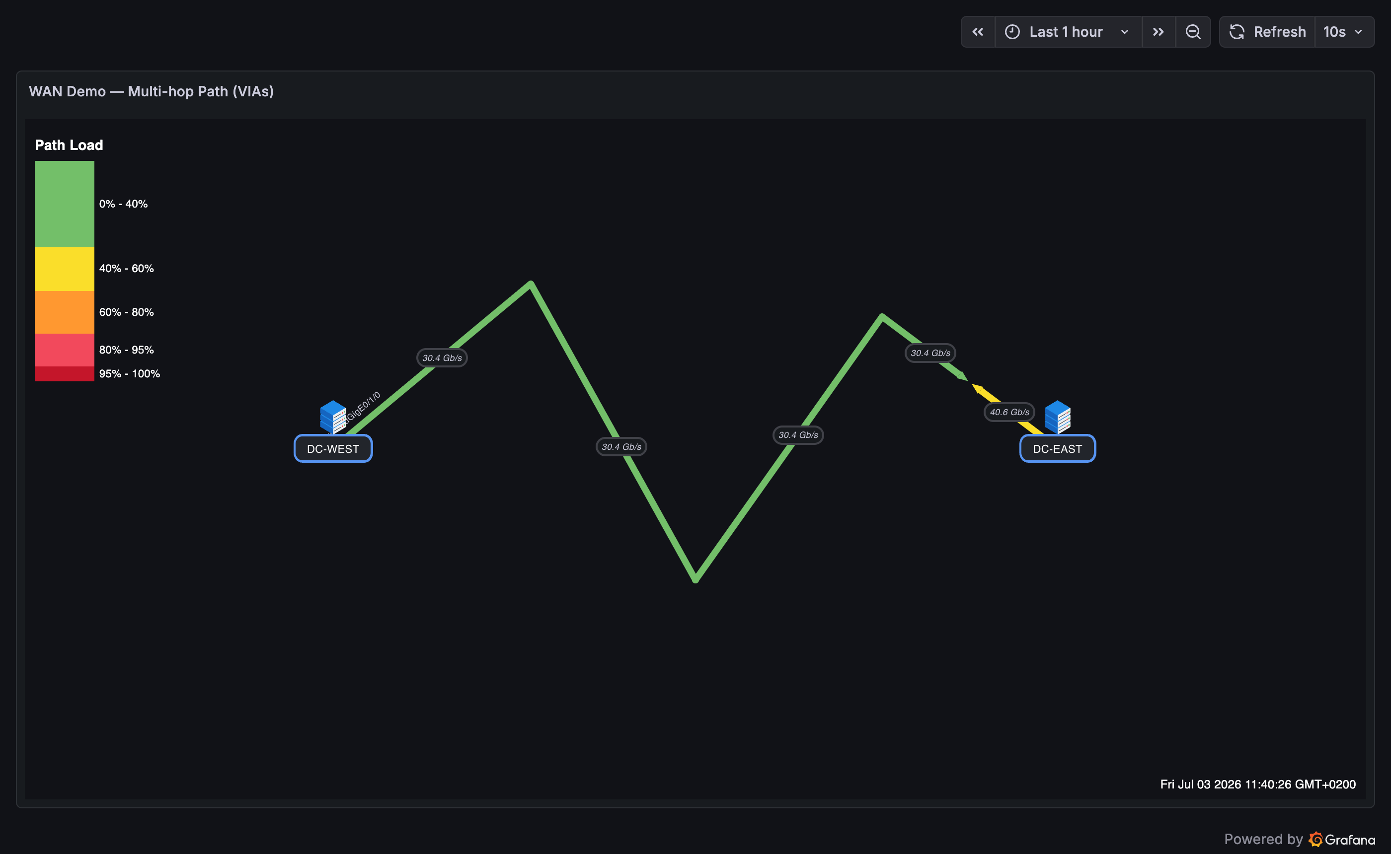
- Create the A and Z nodes and a direct link.
- In edit mode, double-click the link to drop a VIA, then drag it to the bend point.
- Repeat to add more bends. Use Arrow Meeting Point (%) to place the direction arrows on the most meaningful segment.
- Right-click any VIA to remove it later.
Demo: WAN Demo — Multi-hop Path (VIAs) — one DC interconnect routed through three VIA points; the A-side value rides the first segment and the Z-side value the last, exactly as VIA editing produces.
6. Device health overview (status coloring)
Goal: at-a-glance device health without reading numbers.
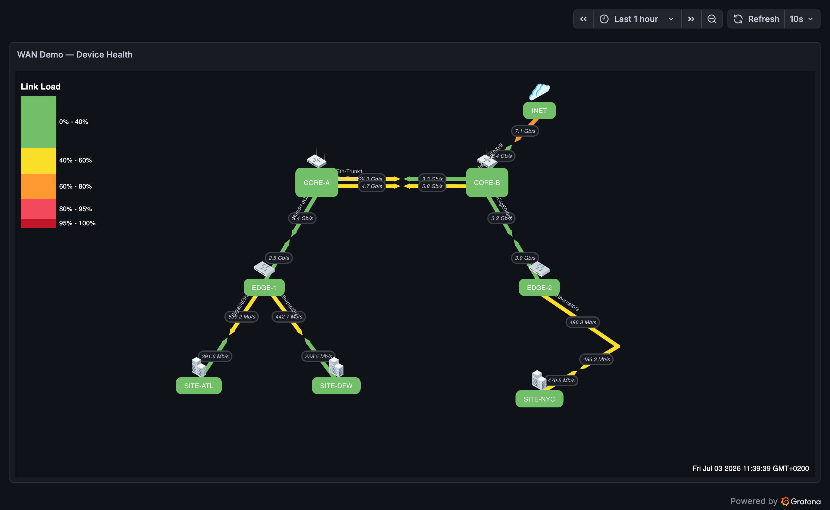
- For each node, open Status and set a Query (e.g.
up, CPU %, temperature). - Add Threshold Mappings (
value ≥ threshold → color) and pick a Color Target (Border / Background / Both). - Optionally add node Tooltip metrics (latency, packet loss, CPU) so hovering shows the detail behind the color.
Demo: WAN Demo — Device Health — every device is colored by packet-loss mappings (green <1%, orange 1–50%, red above); hover any node for its latency/loss tooltip.
7. Parallel links between the same nodes
Goal: show a LAG/port-channel or redundant paths as separate lines.
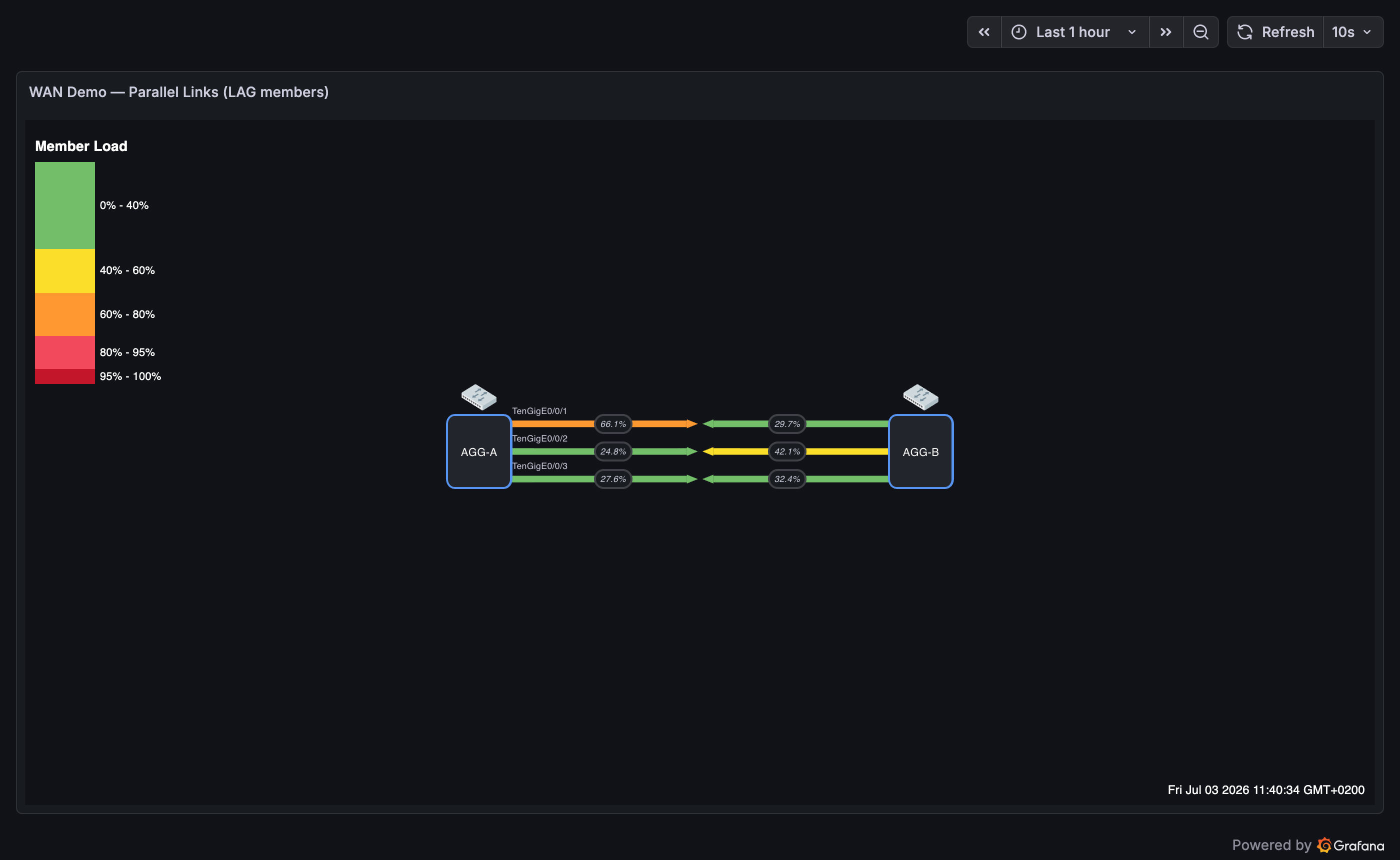
- Add multiple links between the same two nodes.
- Give each a different Link Offset (parallel links) value (e.g.
-8,0,+8) so they spread apart. - Set each link's own query so the members are individually visible.
Demo: WAN Demo — Parallel Links (LAG members) — a three-member LAG with per-member queries, port labels, and utilization percentages; unequal hashing shows one member running hot.
8. Clickable drill-down map
Goal: click a device to open its detailed dashboard.
- Give each node a Dashboard Link (e.g.
/d/abc/switch-detail?var-host=$host). - Use
${var}template variables in labels, queries, and links for dynamic, reusable maps. - In view mode, clicking the node navigates to the target (safely, in a new tab by default).
Demo: the demo dashboards form a drill-down chain — Global Backbone → click NYC → WAN Utilization → click a SITE → Building Floor Plan → click RACK1-TOR → Rack Port Status.
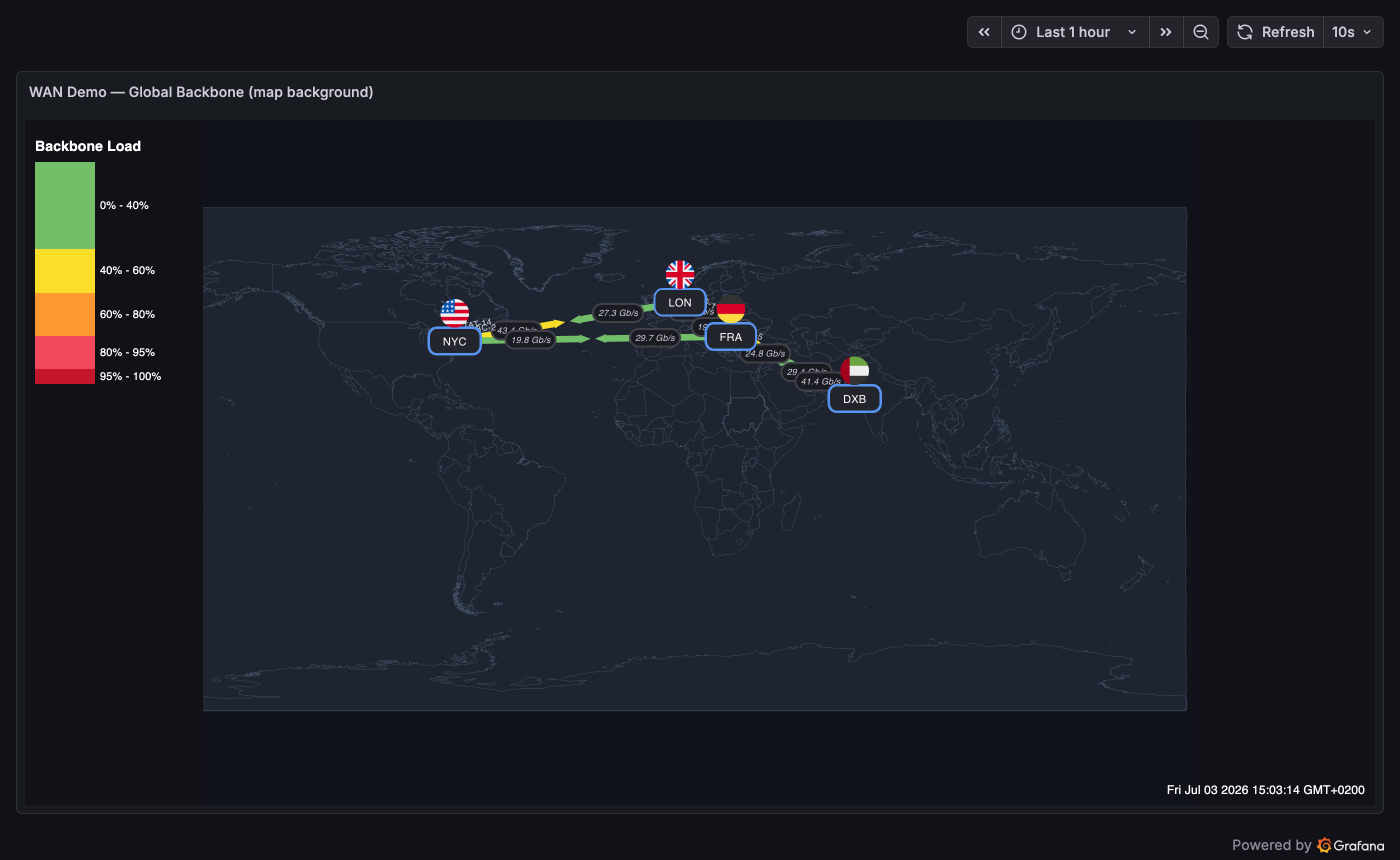
9. Global backbone on a world map
Goal: intercontinental links (e.g. USA ↔ Europe ↔ Middle East) drawn over real geography.
Background image hosting
The background is a URL — any http:// or https:// link works, or drop the file in Grafana's public/ folder and reference it as public/img/<name> (air-gap friendly). data: URLs are rejected. Details: Panel Options → Background.
- Use a world-map image as the Background (public-domain equirectangular SVGs are available on Wikimedia Commons); set Image Fit to
containand enable Move With Map. - Place a node per PoP/city at its location on the map; the bundled Country Flags icon set (ISO two-letter codes) marks each PoP's country.
- Add the submarine/backbone links between them with per-direction queries and capacities; use Port Labels for the cable/system names.
Demo: WAN Demo — Global Backbone (map background) — NYC, London, Frankfurt, and Dubai over a recolored public-domain world map; clicking NYC drills into the regional WAN.
10. Rack / switch port status board
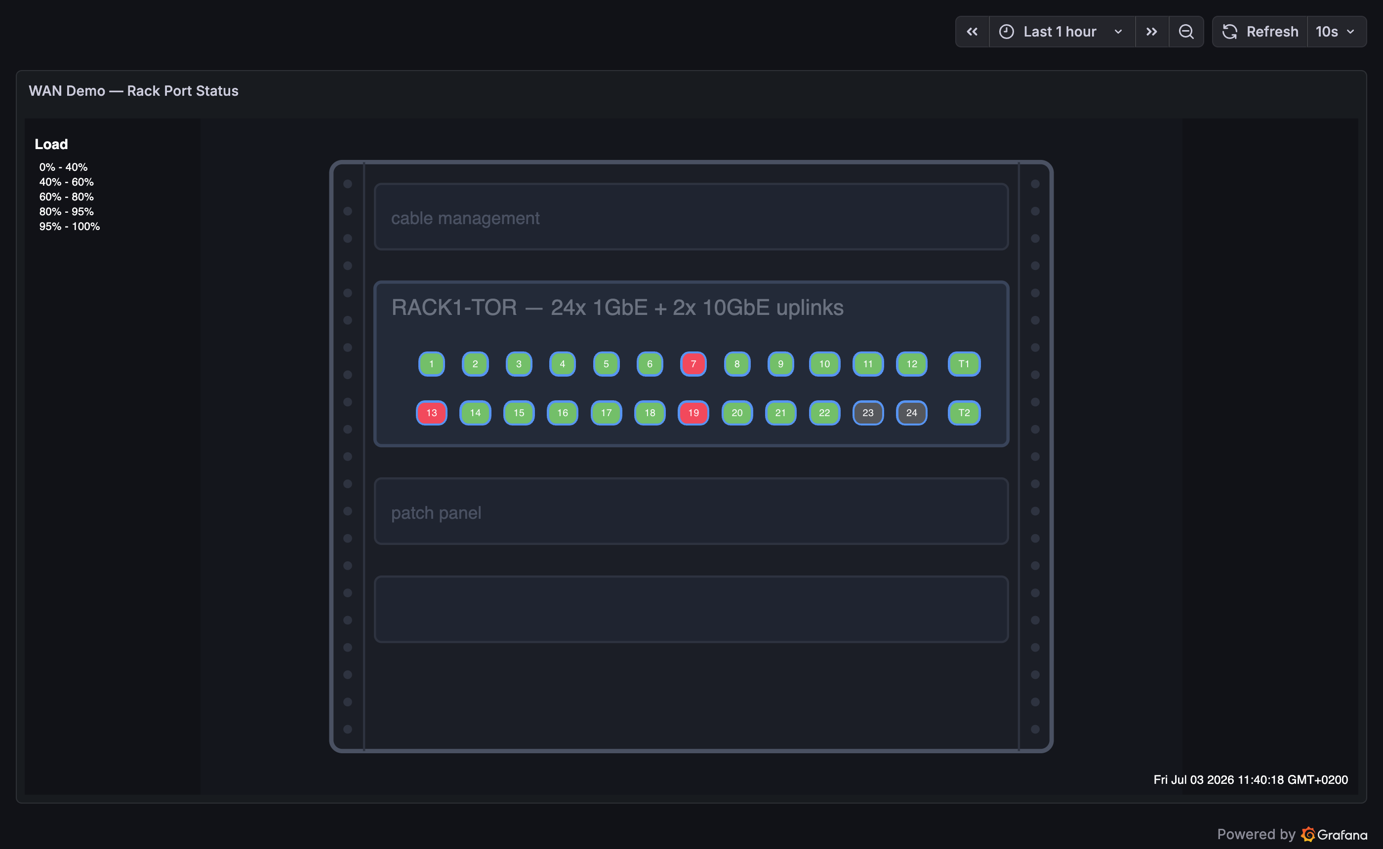
Goal: a faceplate-style board showing every switch port's status at a glance.
Background image hosting
The background is a URL — any http:// or https:// link works, or drop the file in Grafana's public/ folder and reference it as public/img/<name> (air-gap friendly). data: URLs are rejected. Details: Panel Options → Background.
- Use a rack/faceplate drawing as the Background image.
- Add one small node per port (label = port number) positioned over the faceplate; no links needed.
- Set each node's Status Query to that port's status series and add Threshold Mappings — e.g.
0 → red(down),1 → green(up),2 → gray(admin-disabled) — with Color Target = Background.
Demo: WAN Demo — Rack Port Status — 24 access ports plus two 10G uplinks; ports 7/19 are hard down, port 13 flaps every ~5 minutes, 23/24 are admin-disabled.
11. Rack cabling & power redundancy (multi-device rear view)
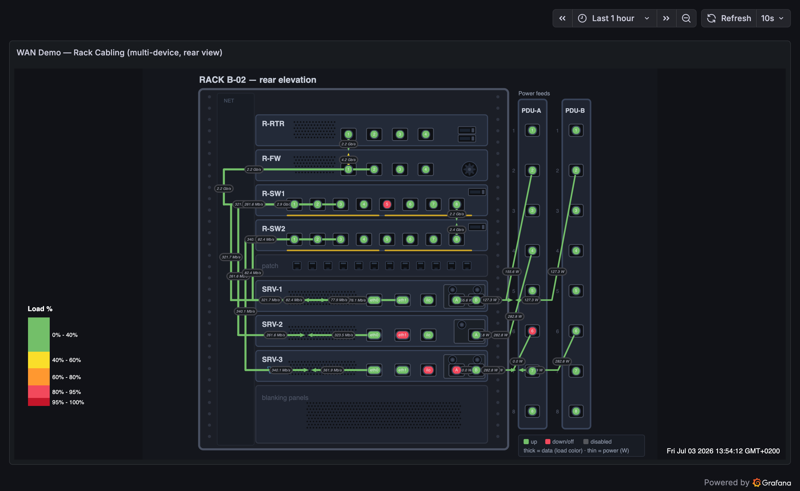
Goal: one rack's rear elevation — router, firewall, switches, servers — with the actual cable runs between ports and the A/B power feeds, so a failed feed or unpatched port is visible at a glance.
Background image hosting
The background is a URL — any http:// or https:// link works, or drop the file in Grafana's public/ folder and reference it as public/img/<name> (air-gap friendly). data: URLs are rejected. Details: Panel Options → Background.
- Draw the rack rear elevation (device faceplates, cable channels, PDU strips) as the Background image with Move With Map enabled.
- Add one small node per port/NIC/PSU-inlet/PDU-outlet, placed over the drawn openings, each with a Status Query and threshold mappings (
0 → red,1 → green,2 → gray). - Draw each network cable as a link between the two port nodes it patches, routed through the cable channel with VIAs; give each cable its live traffic query.
- Draw power cables from PDU outlets to PSU inlets with the PDU outlet as the A side so the arrows lead feed → server; set Units to
wattand use each PSU's per-feed power-draw series on both sides of its cable (e.g.power{feed="A"}on the A-feed cable,{feed="B"}on the B-feed cable) — that way a dead outlet shows 0 W on its own cable while the surviving feed carries the full draw. - Mix dual- and single-supply servers as your rack really is — a dual-fed server survives a dead outlet (its full draw shifts to the B feed and the wattage labels show it); a single-supply server visibly does not have that safety net.
Where power metrics come from
Smart/metered PDUs (APC, Raritan, Vertiv, …) expose per-outlet state, voltage, current, and power over SNMP — scrape them with the Prometheus snmp_exporter. If your PDU is dumb (no metrics), get the wattage from the server side instead: BMC interfaces via ipmi_exporter or Redfish (iDRAC/iLO), or the OS's power sensors via node_exporter's hwmon collectors. The map doesn't care which — it just needs one series per feed.
Demo: WAN Demo — Rack Cabling (multi-device, rear view) — SW1 port 5 down, SRV-2's standby NIC down, and SRV-3's A feed plugged into PDU-A's dead outlet 6: its A cable reads 0 W while the B feed carries the full draw.
12. Dense-map readability & interaction
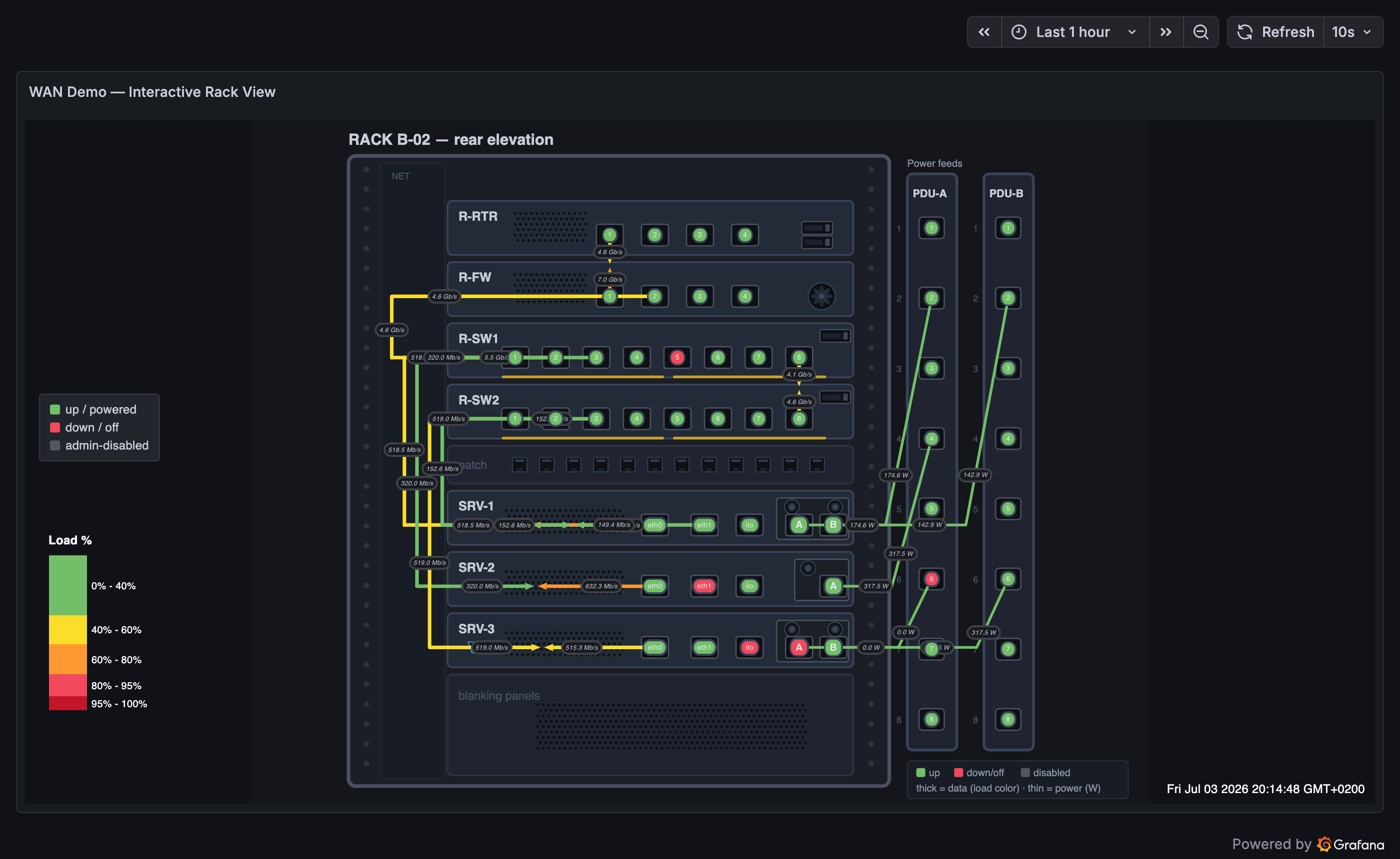
Goal: keep a busy map (dozens of cables, ports, and labels) readable and explorable — highlight what you're looking at, cut label clutter, and explain your colors on the map itself. Requires plugin 1.5.12+.
-
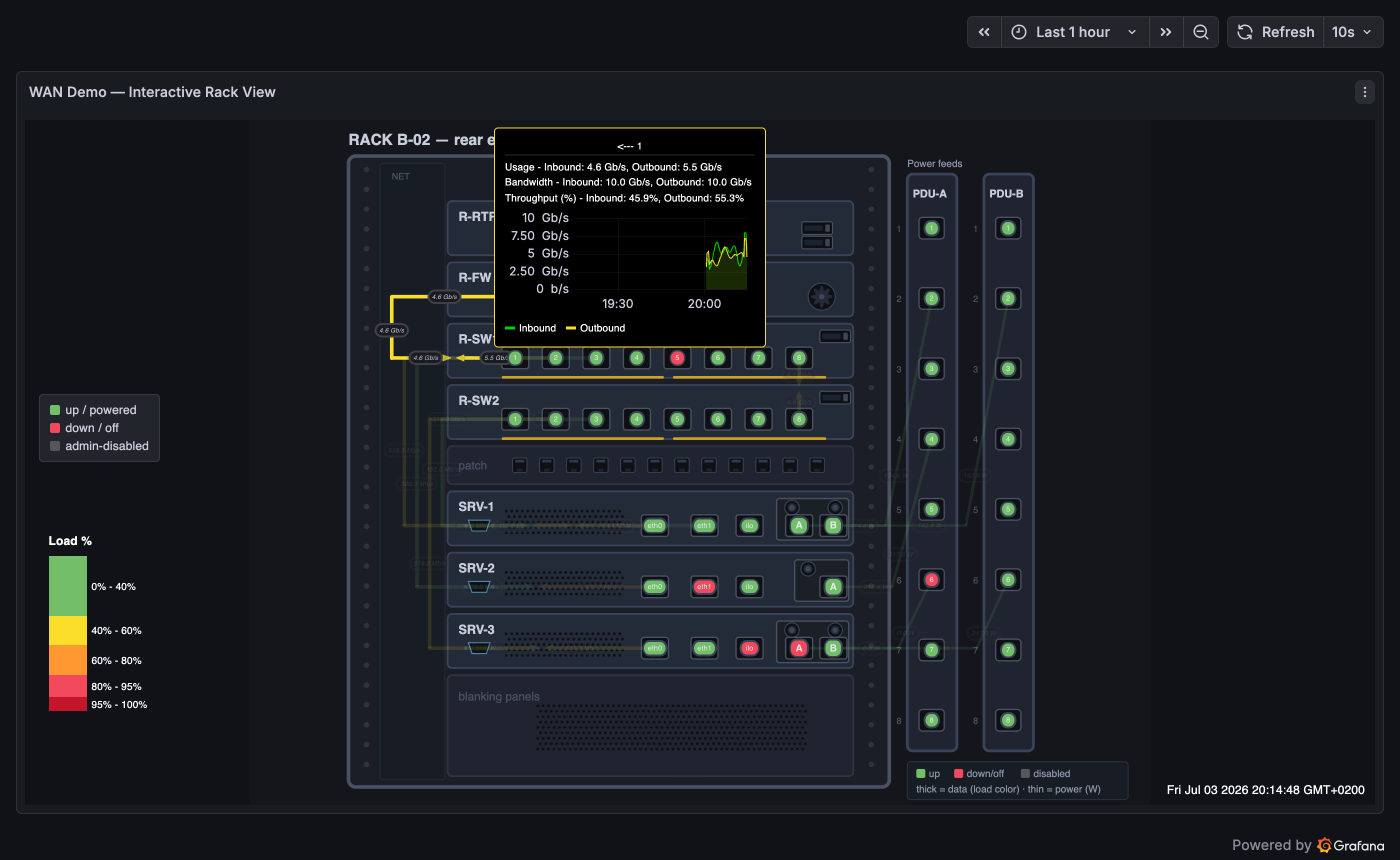
Panel Options → Hover Highlight — hovering a link keeps its whole path (including every VIA segment) at full opacity and fades all other links and value labels, so a single cable can be traced through the densest map:
-
Panel Options → Label Collision Avoidance — overlapping value labels nudge themselves apart along their own links automatically, replacing hand-tuned label offsets.
- Panel Options → Hide Labels When Zoomed Out — value labels disappear once you zoom out past the configured number of scroll steps and return as you zoom in, keeping the overview clean.
- Panel Options → Status Legend — a built-in legend with your own color+label rows (visible top-left in the screenshots), positioned in panel percent coordinates.
- Per link: Single Direction (A → Z) — flows that physically go one way (power feeds, one-way replication) render as one full-length line with a single arrow into the destination and one value label, instead of the two-sided default.
- Per node: Label Font Size / Bold (under the node's Advanced section) — emphasize important labels (here the PSU inlet
A/Bmarkers) while structural labels stay muted.
Demo: WAN Demo — Interactive Rack View — the rack-cabling topology with all six features enabled: hover any cable to trace it, note the one-way power feeds carrying live wattage into each PSU inlet, and zoom out two steps to watch the labels declutter.
13. Animated traffic flow (moving dots)
Goal: make traffic direction and intensity readable at a glance — a link streams dots the way it's carrying traffic, faster and denser as it fills, while a down link visibly stops. Requires plugin 1.6.0+.
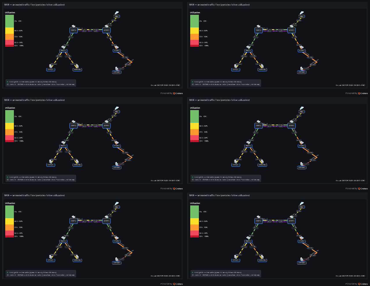
- Panel Options → Animation → Enable Traffic Animation — the master switch (off by default).
- Make sure each animated link has a side query and a bandwidth (fixed or query) — animation reuses the values that already color the link; no extra queries are needed. Utilization = value ÷ bandwidth drives dot speed (
20 + √u·100px/s) and density (1 + round(u·7)dots); dot color inherits the link's threshold color. - Per link → Traffic Animation — leave Inherit to follow the panel switch, or set Enabled to spotlight one flow / Disabled to keep a link static.
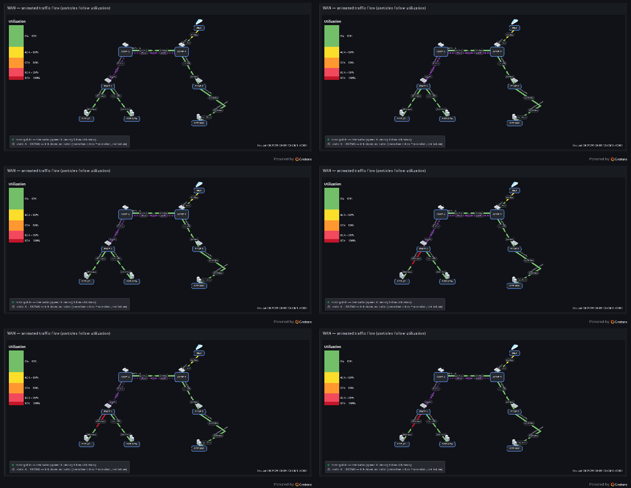
- Add a Status Query so a failed link swaps its dots for static ✕ badges and reads DOWN — traffic can't flow on a broken link.
- Safety is built in: reduced-motion is honored, edit-mode pauses, and Max Animated Links caps large maps. Dots are native SVG animation (compositor-only) so the panel never re-renders per frame.
This is a visualization of metrics you already query — not packet capture. See the full reference (SNMP/Prometheus data flow, PromQL, timeline behavior, accessibility) in Traffic Animation.
It reacts to real data, not a canned animation
The dots, colors, and down-state all follow the live time series. In the demo, forcing the operational status of the CORE-A ↔ EDGE-1 link to 0 (a real interface-down event) makes the plugin drop its dots, dash the line, blink it, stamp both ends DOWN, and draw static ✕ badges — while every healthy link keeps flowing. Restore the feed and it animates again on the next scrape.
Data source setup (Prometheus)
The demo dashboard is fed by the testing stack: a small exporter simulates SNMP interface counters and operational status, Prometheus scrapes them, and the panel binds the resulting series. This is the same shape as a production SNMP path — swap the simulator for snmp_exporter:
  Network device (switch / router / firewall)
     │  interface counters + ifOperStatus  (SNMP)
     ▼
  snmp_exporter (if_mib)          ← demo: a metrics exporter simulating the same series
     │  /metrics  (wm_link_bps, wm_link_status …)
     ▼
  Prometheus  ── scrape ──▶ stores the time series
     │  PromQL:  rate(ifHCOutOctets[2m]) * 8   /   ifOperStatus
     ▼
  Grafana query (per link side + status)
     │  display name = legend
     ▼
  Network Weathermap NG
     • A/Z side value → dot direction, speed, density
     • bandwidth      → utilization → color + dot count
     • status query   → down: dashed line, DOWN, static ✕
Bind it in the link editor: A/Z Side Query = the direction's bits/sec, A/Z Bandwidth = the interface capacity, Status Query = the operational status (wm_link_status{link="…"}, or ifOperStatus{…} in production). See Data Sources → Prometheus for the query/legend details.
Demo: WAN Demo — Animated Traffic Flow — low/medium/high/bidirectional/idle links plus a permanently-down trunk showing ✕ badges next to an animated one, with the built-in legend explaining the glyphs.
Tips that apply everywhere
- Template variables (
$var,${var}) are resolved at draw time in labels, queries, status queries, dashboard links, and bandwidth queries — build one panel that serves many sites. - Export SVG/JSON from the Export section to share diagrams or move a map between panels.
- Keep series display names unique and readable — that's how weathermap matches queries to links/nodes.